scipy.special.fdtr

scipy.special.fdtr(dfn, dfd, x, out=None) = <ufunc 'fdtr'>

F cumulative distribution function.

Returns the value of the cumulative distribution function of the F-distribution, also known as Snedecor’s F-distribution or the Fisher-Snedecor distribution.

The F-distribution with parameters \(d_n\) and \(d_d\) is the distribution of the random variable,

\[X = \frac{U_n/d_n}{U_d/d_d},\]

where \(U_n\) and \(U_d\) are random variables distributed \(\chi^2\), with \(d_n\) and \(d_d\) degrees of freedom, respectively.

Parameters:

dfnarray_like

First parameter (positive float).

dfdarray_like

Second parameter (positive float).

xarray_like

Argument (nonnegative float).

outndarray, optional

Optional output array for the function values

Returns:

yscalar or ndarray

The CDF of the F-distribution with parameters dfn and dfd at x.

See also

fdtrc

F distribution survival function

fdtri

F distribution inverse cumulative distribution

scipy.stats.f

F distribution

Notes

The regularized incomplete beta function is used, according to the formula,

\[F(d_n, d_d; x) = I_{xd_n/(d_d + xd_n)}(d_n/2, d_d/2).\]

Wrapper for a routine from the Boost Math C++ library [1]. The F distribution is also available as scipy.stats.f. Calling fdtr directly can improve performance compared to the cdf method of scipy.stats.f (see last example below).

Array API Standard Support

fdtr has experimental support for Python Array API Standard compatible backends in addition to NumPy. Please consider testing these features by setting an environment variable SCIPY_ARRAY_API=1 and providing CuPy, PyTorch, JAX, or Dask arrays as array arguments. The following combinations of backend and device (or other capability) are supported.

Library	CPU	GPU
NumPy	✅	n/a
CuPy	n/a	✅
PyTorch	✅	⛔
JAX	⚠️ no JIT	⛔
Dask	✅	n/a

See Support for the array API standard for more information.

References

[1]

The Boost Developers. “Boost C++ Libraries”. https://www.boost.org/.

Examples

Try it in your browser!

Calculate the function for dfn=1 and dfd=2 at x=1.

>>> import numpy as np
>>> from scipy.special import fdtr
>>> fdtr(1, 2, 1)
0.5773502691896258

Calculate the function at several points by providing a NumPy array for x.

>>> x = np.array([0.5, 2., 3.])
>>> fdtr(1, 2, x)
array([0.4472136 , 0.70710678, 0.77459667])

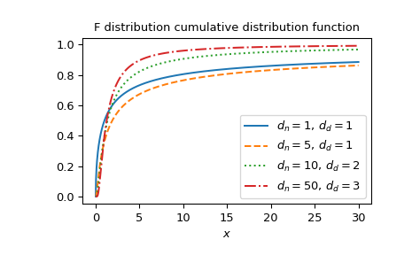
Plot the function for several parameter sets.

>>> import matplotlib.pyplot as plt
>>> dfn_parameters = [1, 5, 10, 50]
>>> dfd_parameters = [1, 1, 2, 3]
>>> linestyles = ['solid', 'dashed', 'dotted', 'dashdot']
>>> parameters_list = list(zip(dfn_parameters, dfd_parameters,
...                            linestyles))
>>> x = np.linspace(0, 30, 1000)
>>> fig, ax = plt.subplots()
>>> for parameter_set in parameters_list:
...     dfn, dfd, style = parameter_set
...     fdtr_vals = fdtr(dfn, dfd, x)
...     ax.plot(x, fdtr_vals, label=rf"$d_n={dfn},\, d_d={dfd}$",
...             ls=style)
>>> ax.legend()
>>> ax.set_xlabel("$x$")
>>> ax.set_title("F distribution cumulative distribution function")
>>> plt.show()

The F distribution is also available as scipy.stats.f. Using fdtr directly can be much faster than calling the cdf method of scipy.stats.f, especially for small arrays or individual values. To get the same results one must use the following parametrization: stats.f(dfn, dfd).cdf(x)=fdtr(dfn, dfd, x).

>>> from scipy.stats import f
>>> dfn, dfd = 1, 2
>>> x = 1
>>> fdtr_res = fdtr(dfn, dfd, x)  # this will often be faster than below
>>> f_dist_res = f(dfn, dfd).cdf(x)
>>> fdtr_res == f_dist_res  # test that results are equal
True

Go BackOpen In Tab