scipy.signal.

minimum_phase

scipy.signal.minimum_phase(h, method='homomorphic', n_fft=None, *, half=True)

Convert a linear-phase FIR filter to minimum phase

Parameters:

harray

Linear-phase FIR filter coefficients.

method{‘hilbert’, ‘homomorphic’}

The provided methods are:

‘homomorphic’ (default)

This method [4] [5] works best with filters with an odd number of taps, and the resulting minimum phase filter will have a magnitude response that approximates the square root of the original filter’s magnitude response using half the number of taps when half=True (default), or the original magnitude spectrum using the same number of taps when half=False.

‘hilbert’

This method [1] is designed to be used with equiripple filters (e.g., from remez) with unity or zero gain regions.

n_fftint

The number of points to use for the FFT. Should be at least a few times larger than the signal length (see Notes).

halfbool

If True, create a filter that is half the length of the original, with a magnitude spectrum that is the square root of the original. If False, create a filter that is the same length as the original, with a magnitude spectrum that is designed to match the original (only supported when method='homomorphic').

Added in version 1.14.0.

Returns:

h_minimumarray

The minimum-phase version of the filter, with length (len(h) + 1) // 2 when half is True or len(h) otherwise.

See also

firwin

firwin2

remez

Notes

Both the Hilbert [1] or homomorphic [4] [5] methods require selection of an FFT length to estimate the complex cepstrum of the filter.

In the case of the Hilbert method, the deviation from the ideal spectrum epsilon is related to the number of stopband zeros n_stop and FFT length n_fft as:

epsilon = 2. * n_stop / n_fft

For example, with 100 stopband zeros and a FFT length of 2048, epsilon = 0.0976. If we conservatively assume that the number of stopband zeros is one less than the filter length, we can take the FFT length to be the next power of 2 that satisfies epsilon=0.01 as:

n_fft = 2 ** int(np.ceil(np.log2(2 * (len(h) - 1) / 0.01)))

This gives reasonable results for both the Hilbert and homomorphic methods, and gives the value used when n_fft=None.

Alternative implementations exist for creating minimum-phase filters, including zero inversion [2] and spectral factorization [3] [4]. For more information, see this DSPGuru page.

References

[1] (1,2)

N. Damera-Venkata and B. L. Evans, “Optimal design of real and complex minimum phase digital FIR filters,” Acoustics, Speech, and Signal Processing, 1999. Proceedings., 1999 IEEE International Conference on, Phoenix, AZ, 1999, pp. 1145-1148 vol.3. DOI:10.1109/ICASSP.1999.756179

[2]

X. Chen and T. W. Parks, “Design of optimal minimum phase FIR filters by direct factorization,” Signal Processing, vol. 10, no. 4, pp. 369-383, Jun. 1986.

[3]

T. Saramaki, “Finite Impulse Response Filter Design,” in Handbook for Digital Signal Processing, chapter 4, New York: Wiley-Interscience, 1993.

[4] (1,2,3)

J. S. Lim, Advanced Topics in Signal Processing. Englewood Cliffs, N.J.: Prentice Hall, 1988.

[5] (1,2)

A. V. Oppenheim, R. W. Schafer, and J. R. Buck, “Discrete-Time Signal Processing,” 3rd edition. Upper Saddle River, N.J.: Pearson, 2009.

Examples

Try it in your browser!

Create an optimal linear-phase low-pass filter h with a transition band of [0.2, 0.3] (assuming a Nyquist frequency of 1):

>>> import numpy as np
>>> from scipy.signal import remez, minimum_phase, freqz, group_delay
>>> import matplotlib.pyplot as plt
>>> freq = [0, 0.2, 0.3, 1.0]
>>> desired = [1, 0]
>>> h_linear = remez(151, freq, desired, fs=2)

Convert it to minimum phase:

>>> h_hil = minimum_phase(h_linear, method='hilbert')
>>> h_hom = minimum_phase(h_linear, method='homomorphic')
>>> h_hom_full = minimum_phase(h_linear, method='homomorphic', half=False)

Compare the impulse and frequency response of the four filters:

>>> fig0, ax0 = plt.subplots(figsize=(6, 3), tight_layout=True)
>>> fig1, axs = plt.subplots(3, sharex='all', figsize=(6, 6), tight_layout=True)
>>> ax0.set_title("Impulse response")
>>> ax0.set(xlabel='Samples', ylabel='Amplitude', xlim=(0, len(h_linear) - 1))
>>> axs[0].set_title("Frequency Response")
>>> axs[0].set(xlim=(0, .65), ylabel="Magnitude / dB")
>>> axs[1].set(ylabel="Phase / rad")
>>> axs[2].set(ylabel="Group Delay / samples", ylim=(-31, 81),
...             xlabel='Normalized Frequency (Nyqist frequency: 1)')
>>> for h, lb in ((h_linear,   f'Linear ({len(h_linear)})'),
...               (h_hil,      f'Min-Hilbert ({len(h_hil)})'),
...               (h_hom,      f'Min-Homomorphic ({len(h_hom)})'),
...               (h_hom_full, f'Min-Homom. Full ({len(h_hom_full)})')):
...     w_H, H = freqz(h, fs=2)
...     w_gd, gd = group_delay((h, 1), fs=2)
...
...     alpha = 1.0 if lb == 'linear' else 0.5  # full opacity for 'linear' line
...     ax0.plot(h, '.-', alpha=alpha, label=lb)
...     axs[0].plot(w_H, 20 * np.log10(np.abs(H)), alpha=alpha)
...     axs[1].plot(w_H, np.unwrap(np.angle(H)), alpha=alpha, label=lb)
...     axs[2].plot(w_gd, gd, alpha=alpha)
>>> ax0.grid(True)
>>> ax0.legend(title='Filter Phase (Order)')
>>> axs[1].legend(title='Filter Phase (Order)', loc='lower right')
>>> for ax_ in axs:  # shade transition band:
...     ax_.axvspan(freq[1], freq[2], color='y', alpha=.25)
...     ax_.grid(True)
>>> plt.show()

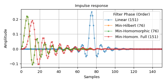
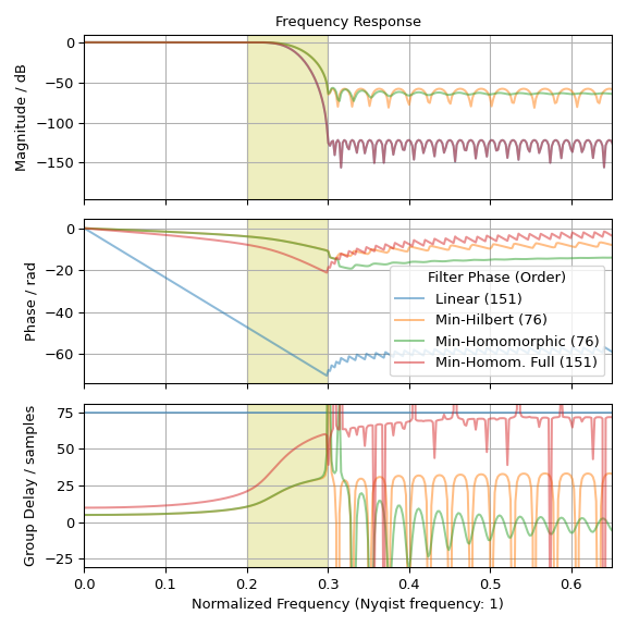
The impulse response and group delay plot depict the 75 sample delay of the linear phase filter h. The phase should also be linear in the stop band–due to the small magnitude, numeric noise dominates there. Furthermore, the plots show that the minimum phase filters clearly show a reduced (negative) phase slope in the pass and transition band. The plots also illustrate that the filter with parameters method='homomorphic', half=False has same order and magnitude response as the linear filter h whereas the other minimum phase filters have only half the order and the square root of the magnitude response.

Go BackOpen In Tab