scipy.signal.

ZoomFFT#

class scipy.signal.ZoomFFT(n, fn, m=None, *, fs=2, endpoint=False)[source]#

Create a callable zoom FFT transform function.

This is a specialization of the chirp z-transform (CZT) for a set of equally-spaced frequencies around the unit circle, used to calculate a section of the FFT more efficiently than calculating the entire FFT and truncating.

Parameters:

nint: The size of the signal.
fnarray_like: A length-2 sequence [f1, f2] giving the frequency range, or a scalar, for which the range [0, fn] is assumed.
mint, optional: The number of points to evaluate. Default is n.
fsfloat, optional: The sampling frequency. If fs=10 represented 10 kHz, for example, then f1 and f2 would also be given in kHz. The default sampling frequency is 2, so f1 and f2 should be in the range [0, 1] to keep the transform below the Nyquist frequency.
endpointbool, optional: If True, f2 is the last sample. Otherwise, it is not included. Default is False.

Methods

`__call__`(x, *[, axis])	Calculate the chirp z-transform of a signal.
`points`()	Return the points at which the chirp z-transform is computed.

Returns:

fZoomFFT: Callable object f(x, axis=-1) for computing the zoom FFT on x.

See also

zoom_fft: Convenience function for calculating a zoom FFT.

Notes

The defaults are chosen such that f(x, 2) is equivalent to fft.fft(x) and, if m > len(x), that f(x, 2, m) is equivalent to fft.fft(x, m).

Sampling frequency is 1/dt, the time step between samples in the signal x. The unit circle corresponds to frequencies from 0 up to the sampling frequency. The default sampling frequency of 2 means that f1, f2 values up to the Nyquist frequency are in the range [0, 1). For f1, f2 values expressed in radians, a sampling frequency of 2*pi should be used.

Remember that a zoom FFT can only interpolate the points of the existing FFT. It cannot help to resolve two separate nearby frequencies. Frequency resolution can only be increased by increasing acquisition time.

These functions are implemented using Bluestein’s algorithm (as is scipy.fft). [2]

References

[1]

Steve Alan Shilling, “A study of the chirp z-transform and its applications”, pg 29 (1970) https://krex.k-state.edu/dspace/bitstream/handle/2097/7844/LD2668R41972S43.pdf

[2]

Leo I. Bluestein, “A linear filtering approach to the computation of the discrete Fourier transform,” Northeast Electronics Research and Engineering Meeting Record 10, 218-219 (1968).

Examples

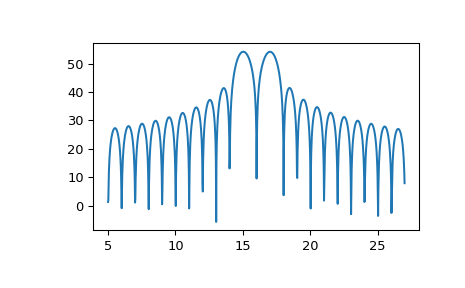
To plot the transform results use something like the following:

>>> import numpy as np
>>> from scipy.signal import ZoomFFT
>>> t = np.linspace(0, 1, 1021)
>>> x = np.cos(2*np.pi*15*t) + np.sin(2*np.pi*17*t)
>>> f1, f2 = 5, 27
>>> transform = ZoomFFT(len(x), [f1, f2], len(x), fs=1021)
>>> X = transform(x)
>>> f = np.linspace(f1, f2, len(x))
>>> import matplotlib.pyplot as plt
>>> plt.plot(f, 20*np.log10(np.abs(X)))
>>> plt.show()

../../_images/scipy-signal-ZoomFFT-1.png