scipy.linalg.

lstsq#

scipy.linalg.lstsq(a, b, cond=None, overwrite_a=False, overwrite_b=False, check_finite=True, lapack_driver=None)[source]#

Compute least-squares solution to equation Ax = b.

Compute a vector x such that the 2-norm |b - A x| is minimized.

The documentation is written assuming array arguments are of specified “core” shapes. However, array argument(s) of this function may have additional “batch” dimensions prepended to the core shape. In this case, the array is treated as a batch of lower-dimensional slices; see Batched Linear Operations for details.

Parameters:

a(M, N) array_like: Left-hand side array
b(M,) or (M, K) array_like: Right hand side array
condfloat, optional: Cutoff for ‘small’ singular values; used to determine effective rank of a. Singular values smaller than cond * largest_singular_value are considered zero.
overwrite_abool, optional: Discard data in a (may enhance performance). Default is False.
overwrite_bbool, optional: Discard data in b (may enhance performance). Default is False.
check_finitebool, optional: Whether to check that the input matrices contain only finite numbers. Disabling may give a performance gain, but may result in problems (crashes, non-termination) if the inputs do contain infinities or NaNs.
lapack_driverstr, optional: Which LAPACK driver is used to solve the least-squares problem. Options are 'gelsd', 'gelsy', 'gelss'. Default ('gelsd') is a good choice. However, 'gelsy' can be slightly faster on many problems. 'gelss' was used historically. It is generally slow but uses less memory.

Added in version 0.17.0.

Returns:

x(N,) or (N, K) ndarray: Least-squares solution.
residues(K,) ndarray or float: Square of the 2-norm for each column in b - a x, if M > N and rank(A) == n (returns a scalar if b is 1-D). Otherwise a (0,)-shaped array is returned.
rankint: Effective rank of a.
s(min(M, N),) ndarray or None: Singular values of a. The condition number of a is s[0] / s[-1].

Raises:

LinAlgError: If computation does not converge.
ValueError: When parameters are not compatible.

See also

scipy.optimize.nnls: linear least squares with non-negativity constraint

Notes

When 'gelsy' is used as a driver, residues is set to a (0,)-shaped array and s is always None.

Examples

>>> import numpy as np
>>> from scipy.linalg import lstsq
>>> import matplotlib.pyplot as plt

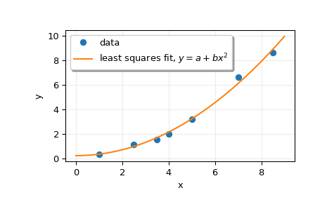
Suppose we have the following data:

>>> x = np.array([1, 2.5, 3.5, 4, 5, 7, 8.5])
>>> y = np.array([0.3, 1.1, 1.5, 2.0, 3.2, 6.6, 8.6])

We want to fit a quadratic polynomial of the form y = a + b*x**2 to this data. We first form the “design matrix” M, with a constant column of 1s and a column containing x**2:

>>> M = x[:, np.newaxis]**[0, 2]
>>> M
array([[  1.  ,   1.  ],
       [  1.  ,   6.25],
       [  1.  ,  12.25],
       [  1.  ,  16.  ],
       [  1.  ,  25.  ],
       [  1.  ,  49.  ],
       [  1.  ,  72.25]])

We want to find the least-squares solution to M.dot(p) = y, where p is a vector with length 2 that holds the parameters a and b.

>>> p, res, rnk, s = lstsq(M, y)
>>> p
array([ 0.20925829,  0.12013861])

Plot the data and the fitted curve.

>>> plt.plot(x, y, 'o', label='data')
>>> xx = np.linspace(0, 9, 101)
>>> yy = p[0] + p[1]*xx**2
>>> plt.plot(xx, yy, label='least squares fit, $y = a + bx^2$')
>>> plt.xlabel('x')
>>> plt.ylabel('y')
>>> plt.legend(framealpha=1, shadow=True)
>>> plt.grid(alpha=0.25)
>>> plt.show()